Prediction
Both classification and regression models implement tools for prediction. Classifiers provide predict_proba (probabilities) and predict (labels), while regressors provide predict (continuous values). All derive predictions based on an ensemble of local models.
The prediction process works as follows:
For a new location on which you want a prediction, identify local models within the bandwidth used to train the model.
Apply the kernel function used to train the model to derive weights of each of the local models.
Make prediction using each of the local models in the bandwidth.
Make weighted average of predictions based on the kernel weights.
For classifiers, normalize the result to ensure sum of probabilities is 1.
Classification prediction
See that in action with a classifier:
import geopandas as gpd
from geodatasets import get_path
from sklearn import metrics
from sklearn.model_selection import train_test_split

from gwlearn.ensemble import GWRandomForestClassifier
Get sample data
gdf = gpd.read_file(get_path("geoda.ncovr")).to_crs(5070)

gdf['point'] = gdf.representative_point()
gdf = gdf.set_geometry('point')

y = gdf["FH90"] > gdf["FH90"].median()
X = gdf.iloc[:, 9:15]
Leave out some locations for prediction later.
X_train, X_test, y_train, y_test, geom_train, geom_test = train_test_split(X, y, gdf.geometry, test_size=.1)
Fit the model using the training subset. If you plan to do the prediction, you need to store the local models, which is False by default. When set to True, all the models are kept in memory, so be careful with large datasets. If given a path, all the models will be stored on disk instead, freeing the memory load.
gwrf = GWRandomForestClassifier(
    geometry=geom_train,
    bandwidth=250,
    fixed=False,
    keep_models=True,
)
gwrf.fit(
    X_train,
    y_train,
)
GWRandomForestClassifier(bandwidth=250,
                         geometry=1989    POINT (-384564.533 1369397.395)
2659        POINT (82854.77 892472.294)
275     POINT (1778051.919 2632546.856)
1967    POINT (1004467.569 1443277.098)
902      POINT (723688.803 1954767.539)
                     ...
939     POINT (1472608.546 2016499.638)
1433     POINT (575941.177 1692254.138)
2754     POINT (-231950.603 796277.137)
1309      POINT (387282.83 1733563.097)
942     POINT (1651190.784 2062911.326)
Name: point, Length: 2776, dtype: geometry,
                         keep_models=True)
In a Jupyter environment, please rerun this cell to show the HTML representation or trust the notebook. On GitHub, the HTML representation is unable to render, please try loading this page with nbviewer.org.
Parameters
| bandwidth | 250 | |
| fixed | False | |
| kernel | 'bisquare' | |
| include_focal | False | |
| geometry | 1989 POINT...type: geometry | |
| graph | None | |
| n_jobs | -1 | |
| fit_global_model | True | |
| strict | False | |
| keep_models | True | |
| temp_folder | None | |
| batch_size | None | |
| min_proportion | 0.2 | |
| undersample | False | |
| leave_out | None | |
| random_state | None | |
| verbose | False |
Now, you can use the test subset to get the prediction. Note that given the prediction is pulled from an ensemble of local models, it is not particularly performant. However, it shall be spatially robust.
proba = gwrf.predict_proba(X_test, geometry=geom_test)
proba
| False | True | |
|---|---|---|
| 805 | 0.811815 | 0.188185 |
| 1704 | 0.096184 | 0.903816 |
| 2872 | 0.833818 | 0.166182 |
| 394 | 0.350391 | 0.649609 |
| 2569 | 0.053624 | 0.946376 |
| ... | ... | ... |
| 2231 | 0.077666 | 0.922334 |
| 2682 | 0.251958 | 0.748042 |
| 1263 | 0.992466 | 0.007534 |
| 2782 | 0.103060 | 0.896940 |
| 2352 | 0.135677 | 0.864323 |
309 rows × 2 columns
You can then check the accuracy of this prediction. Note that similarly to fitting, there might be locations that return NA, if all of the local models within its bandwidth are not fitted.
gpd.GeoDataFrame(proba, geometry=geom_test).plot(True, missing_kwds=dict(color='red')).set_axis_off()
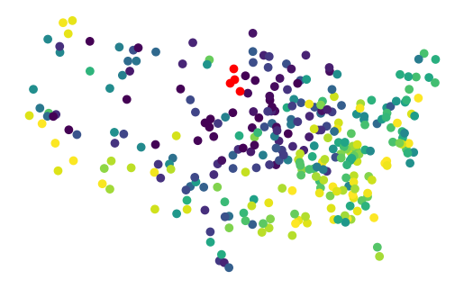
That one red dot, is in the middle of unfittable area.
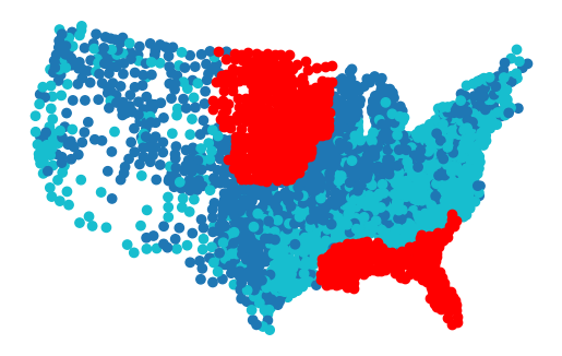
geom_train.to_frame().plot(gwrf.pred_, missing_kwds=dict(color='red')).set_axis_off()
Filter it out and measure the performance on the left-out sample.
na_mask = proba.isna().any(axis=1)

pred = proba[~na_mask].idxmax(axis=1).astype(bool)

metrics.accuracy_score(y_test[~na_mask], pred)
0.819672131147541
Prediction with regressors
Regression models also implement predict method following the same logic as classifiers. Let’s see that in action with a GWLinearRegression.
from gwlearn.linear_model import GWLinearRegression
Prepare the data with a continuous target variable.
y_reg = gdf["FH90"]  # Use the continuous variable directly

X_train_reg, X_test_reg, y_train_reg, y_test_reg, geom_train_reg, geom_test_reg = train_test_split(
    X, y_reg, gdf.geometry, test_size=0.1, random_state=42
)
Fit the regression model with keep_models=True to enable prediction.
gwrf_reg = GWLinearRegression(
    geometry=geom_train_reg,
    bandwidth=250,
    fixed=False,
    keep_models=True,
)
gwrf_reg.fit(
    X_train_reg,
    y_train_reg,
)
GWLinearRegression(bandwidth=250,
                   geometry=2641        POINT (129880.19 911766.583)
1047    POINT (-2212037.741 2151301.959)
594     POINT (-2165220.928 2370376.655)
610       POINT (286075.006 2085516.869)
80      POINT (-1931884.497 2981305.084)
                      ...
1638     POINT (-287577.792 1576667.845)
1095      POINT (297604.304 1833993.506)
1130       POINT (1101533.1 1883572.176)
1294     POINT (1663727.596 1895694.295)
860      POINT (-319662.283 1956527.582)
Name: point, Length: 2776, dtype: geometry,
                   keep_models=True)
In a Jupyter environment, please rerun this cell to show the HTML representation or trust the notebook. On GitHub, the HTML representation is unable to render, please try loading this page with nbviewer.org.
Parameters
| bandwidth | 250 | |
| fixed | False | |
| kernel | 'bisquare' | |
| include_focal | True | |
| geometry | 2641 P...type: geometry | |
| graph | None | |
| n_jobs | -1 | |
| fit_global_model | True | |
| strict | False | |
| keep_models | True | |
| temp_folder | None | |
| batch_size | None | |
| verbose | False |
Make predictions on the test set using the predict method.
pred_reg = gwrf_reg.predict(X_test_reg, geometry=geom_test_reg)
pred_reg
1505    11.515287
2399    13.605516
1814    13.033449
511      9.026350
1565    12.208486
          ...
650     11.322007
176      7.086847
2268    17.239779
2151    13.479579
903     10.796190
Length: 309, dtype: float64
Visualize the predicted values spatially.
gpd.GeoDataFrame({"prediction": pred_reg}, geometry=geom_test_reg).plot(
    "prediction", legend=True
).set_axis_off()
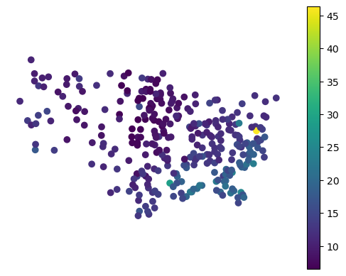
Evaluate the prediction performance using common regression metrics.
print(f"R2 score: {metrics.r2_score(y_test_reg, pred_reg):.3f}")
print(f"RMSE: {metrics.root_mean_squared_error(y_test_reg, pred_reg):.3f}")
R² score: 0.645
RMSE: 3.348